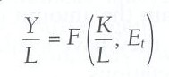
Economists have measured large differences in GDP per capita over time and across countries. To explain such differences in GDP per capita, a growth function has been proposed by several economists; the growth function stems from the statistical observation that output of the economy increases with the labor force, the amount of technology it uses, and its efficiency in using the technology that is available.
Thus the simplest form of growth function relates output/labor Y/L ratio with capital/labor K/L ratio and a measure E, defined as the efficiency of labor. The growth function says that output/labor Y/L is some function F of capital/labor K/L and the efficiency of labor E at a period of time t:
This expression does not specify which function it is; and unless such a specification is given the concept is not very useful. However, parabolic functions are most common in modelling; so a parabolic function of the style, :
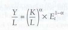
can be useful; the capital/labor K/L ratio and the efficiency of labor are given weights of influence of a and 1-a respectively.
This growth formula allows for an infinity of growth models eg. any series of statistical data may be modelised using the appropriate value of a and a value of E that enables matching the model with actual statistical data.
But let us first start by disregarding the value of E, or E=0 so
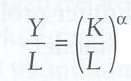
If a = 0.25, then the function is
(Y/L) = (K/L)0.25
Suppose that we are interested in the percentage difference in output/labor Y/L between two points in time or between two countries. If we take the decimal logs of both sides of the production function, we have:
log(Y/L) = 0.25 log(K/L)
Thinking of this as a relation between percentage changes, it says that for a 1% difference in the capital-labor ratio, we should get a 0.25% point difference in output per worker. Conversely, if we observe that one country has 10% higher output per worker than another country, then we would expect the more productive country to have 40% more capital per worker.
In theory, differences in the capital/labor K/L ratio should explain all of the differences in output/labor Y/L.
The capital/labor ratio K/L certainly is important. Countries increase this ratio through capital accumulation. This means that a large share of output Y goes to investment, which helps to increase the stock of capital, thus the capital available to workers. Most of the countries with high rates of labor productivity have investment shares of more than 20% of output. Conversely, the majority of low-productivity countries have investment rates below 20%.
However, differences in the capital/labor ratio explain no more than half of the differences in output per worker Y/L. This is true whether you are trying to explain output per worker Y/L over time in one country or you are trying to explain differences in output per worker Y/L between different countries.
Another way of putting this is that the differences in output per worker Y/L are larger than what you would predict on the basis of the capital-labor ratio K/L. In the United States, growth in output/labor Y/L has been greater than what one would have predicted based on the increase in the capital/labor ratio K/L. Moreover, the difference between output/labor Y/L in the U.S. and in other countries is greater than what one would predict on the basis of differences in the capital/labor ratio.
This phenomenon of unexplained differences in output/labor Y/L was first discovered in the 1950's, and was dubbed "the residual." The residual is so important that we need to find a place for it in the production function. DeLong's Macroeconomics textbook calls it E, the efficiency of labor. Using this formulation, the production function is
and with a value of a = 0.5, the growth function becomes
(Y/L) = (K/L)0.5E0.5
in which output/labor Y/L of an economy is explained 50% by capital/labor ratio K/L and 50% by the efficency of that labor E.
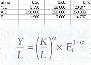
Thus the model shows with a low value of a (0.25), E is high (14800), with a high value of a (0.75) E is very low (52), and with a median value of a (0.50), E is 3600.
In reality, the appropriate values of E and a are those that enable to achieve the best fit between the model and the actual statistical data.
This new construct, the efficiency of labor, gives us another element in the equation. Growth in output per worker is explained as a weighted average of the growth in capital per worker and growth in the efficiency of labor. Taking logs of both sides of the new production function gives
log(Y/L) = 0.25log(K/L) + 0.75log(E)
Now, we have an equation that says that economic growth is a weighted average of growth in the capital-labor ratio and growth in the efficiency of labor. Keep in mind that the efficiency of labor is just what is needed to enable a production function to fit the observed data on output per worker and capital per worker.
Having coined the term "efficiency of labor," economists have to produce some analysis of what determines it. Some plausible factors include:
Of these factors, the only one that has a ready scale of measurement is education. In fact, some of the differences in the efficiency of labor across time and across countries can be explained by differences in the average years of schooling per worker. However, education does not explain enough to make us comfortable that it is the overwhelming factor that determines E.
Knowledge is an important factor in explaining differences in E over time. We simply know things today that we did not know years ago. For example, even if we lost all of our medical equipment and our doctors, we would still know much more about sanitation and health than people did hundreds of years ago.
Some of our knowledge is scientific and technical. Other knowledge is more prosaic. When you start a new job, you typically are given a formal orientation, company manuals, and help from senior employees who through trial and error have learned better ways of doing the work. All of this knowledge, from abstract science to everyday experience, contributes to E.
Some knowledge is in the public domain, and some knowledge is proprietary. Most scientific knowledge is available to anyone who can understand it. However, other knowledge, from the formula for Coke to the source code for Microsoft software, is considered a secret by its corporate owners.
Because most knowledge is in the public domain, knowledge does not provide a promising explanation for variations in E across countries. Even proprietary knowledge is not limited to a single country. For example, Coke has manufacturing plants throughout the world, so that its secret formula is used by workers everywhere.
When we attempt to explain differences in the efficiency of labor in different countries, economists almost inevitably are forced to focus on differences in economic, political, and social systems. The contrast that DeLong draws between output per worker in neighboring pairs of Communist and non-Communist countries certainly underlines this issue.
The production function provides a framework for accounting for growth. It leads to an approach that subdivides growth into two components--the capital-labor ratio and the efficiency of labor.
The efficiency of labor is constructed indirectly, based on the residual that results from trying explain differences in output per worker on the basis of differences in the capital-labor ratio. Economists believe that the efficiency of labor is affected by education, knowledge, and the social system.
When the Industrial Revolution broke out of the Malthusian trap, economies began to accumulate capital goods. In order to accumulate capital, you have to save. This means that you cannot consume all of your output.
[1] S = 5%K
Let us define the savings rate "s" to be the ratio of savings to output, s=S/Y.
and let us write equation [1] with "s", we have:
[2] s = S/Y = 5%K/Y
Equation [2] says, that to maintain output constant, we need a savings rate "s" that equals the rate of depreciation (5%) times the capital/output ratio K/Y.
Now, if we want to have high labor productivity, we need a high ratio of capital to output, and therefore we need a high savings rate "s". Thus, we would expect to find a relationship between countries with high savings rates and countries with high productivity, and this is indeed what Brad DeLong found when he indicated that countries with high productivity tend to have saving rates over 20%.
Suppose that we want the capital stock to grow at a rate of 2%. In that case, we need
[3] S = 5%K + 2%K = 7%K
Or, in terms of s and K/Y,
[4] s = 5%K/Y + 2%K/Y = 7%K/Y
Let "d" be depreciation, "k" be capital-output ratio K/Y, and "x" be growth rate of capital DK/K, then we can write
[5] s = dk + xk
To see how the saving rate affects the growth rate of capital, we can solve equation [5] for x, the growth rate of capital.
[6] x = DK/K = s/k - d
If the labor force is growing at a rate n%, then the capital/labor ratio will grow at the rate of x%-n%. For example, if:
Then we have
[7] x - n = s/k - d - n = 25%/2.5 - 5% -1% = 4%
which says that capital/labor ratio grows at 4 percent per year. In a moment, when I discuss balanced growth, I will argue that this is not a reasonable long-term growth rate for the capital/labor ratio.
We are interested in the growth rate of labor productivity, Y/L. To look at productivity, we return to the production function that we used in the growth accounting lesson.
[8] (Y/L) = (K/L)0.25E0.75
where E is the efficiency of labor. When we took logs of both sides, we obtained an equation for the growth rate of productivity. If y is the growth rate of output and n is the growth rate of the labor force, then the growth rate of productivity is y-n. Letting g be the symbol for the growth rate of E, the efficiency of labor, we have
[9] y - n = 0.25(x - n) + 0.75g
When we made numerical assumptions in equation [7], we found that x-n = 4%. Plugging this into equation [9] and assuming that the growth rate of the efficiency of labor, g, is 2%, we have
[10] y - n = 0.25(4%) + .75(2%) = 2.5%
Thus, the assumptions about saving rate, depreciation, and so forth imply growth in labor productivity of 2.5% per year.
Economists define a balanced growth path as a path along which capital and output grow at the same rate. The alternatives to a balanced growth path are not sustainable. If capital grows more slowly than output, then the capital stock will eventually drop to zero. If capital grows more quickly than output, then the share of output that you set aside for capital goods will increase until you reach the point where the amount available for consumption is zero.
Looking at equation [9], the only way that x and y can be equal is if
[11] g = x - n
That is, for balanced growth, the growth rate of the efficiency of labor must be matched by the growth rate of capital minus the growth rate of the labor force.
The requirement for balanced growth implies that there is only one sustainable ratio of capital to ouput. That is, there is only one ratio of capital to output, k that is consistent with a balanced growth path. Using equations [11] and [7] we have
[12] g = x - n = s/k - d - n
We can solve this equation for a balanced-growth value for k, given the other parameters. Using s = 25%, g = 2%, n = 1% and d = 5%, we have
[13] k = s/(g + n + d) = 0.25/(2%+1%+5%) = 3.125
Therefore, the balanced-growth capital-output ratio is 3.125. If the capital-output ratio happens to be above this level, the savings rate is not high enough to maintain it, and the ratio will tend to fall back to 3.125. Conversely, if the capital-output ratio happens to start out below the balanced-growth level, the savings rate is high enough to generate capital accumulation until the ratio rises back to 3.125. Back at equation [10] when we computed labor productivity growth, we had assumed earlier an arbitrary capital-output ratio of 2.5. Now, we know that this is not a balanced-growth ratio given the saving rate, depreciation rate, and other assumed parameters. Using the balanced-growth ratio of 3.125 in equation [7] gives
[7'] x - n = 0.25/3.125 - 5% - 1% = 2%
Putting this into [10], we have
[10'] y - n = 0.25(2%) + 0.75(2%) = 2%
What we have found is that on a balanced growth path, output per worker and capital per worker grow at the same rate as the efficiency of labor. In our example, this is 2% per year.
Some of the more important ideas about economic growth are based on mathematical models. Let us review what we can learn from mathematical growth models.
The Harrod-Domar growth model gives some insights into the dynamics of growth. We want a method of determining an equilibrium growth rate g for the economy. Let Y be GDP and S be savings.
The level of savings S is a proportion of the level of output Y, say S = sY where s is the propensity to save. The level of capital K needed to produce an output Y is given by the equation K=σY where σ designates the capital/output ratio K/Y.
Investment is a very important variable for the economy because Investment has a double role. Investment I represents an important component of the demand for the output of the economy as well as an increase in the capital stock. Thus Investment I is DK = σDY.
For equilibrium there must be a balance between the supply of savings and the demand for increasing the capital stock. This balance reduces to I = S.
Thus, I = ΔK = σΔY
and I = S = sY
so
σΔY = sY.
Therefore the equilibrium rate of growth ΔY/Y which we call g, is given by:
ΔY/Y = s/σ = g
In other words, the equilibrium growth rate of output is equal to ratio of the propensity of savings s = S/Y and of the capital/output ratio σ = K/Y. This is a very significant result. It tells us that growth in the capacity of the economy to produce is determined by matching the supply of savings and the demand for increasing the capital stock of the economy.
Consider the following numerical example. Suppose the economy is currently operating at an output level of Y/L = 30 000 per year and has a capital-output ratio σ = K/Y = 3. This means the capital stock is 90 000. Assume the savings rate s=25% and the propensity to consume output Y is 75%. Savings rate s=25% includes business and public savings as well as household savings.
The Harrod-Domar growth model tells that the equilibrium growth rate is g = 25%/3 = 8.33%; i.e., the economy can grow at 8.33% per year. We can now check this result with actual aritmetic calculations. We shall calculate from two ends:
At the current output level of Y/L = 30000, the level of saving is 25%*30000=7500. The growth of output is g = 8.33%*30000 = 2500 and with a capital-output ratio of 3 the additional capital required to produce the additional output of 2500 is 3*2500=7500. This is the investment required in order to increase capacity by the right amount and, this is equal to the amount of saving available in the economy ie. 7500. So the balanced growth model requires that Investment equals Saving and the new output Y/L is 30000+2500=32500.
We must check that there is adequate aggregate demand next year to absorb the new production level of 30000+2500=32500. At that level of income, consumer demand is 75% of 32500, so 24375. The level of investment the next year under the assumed equilibrium growth conditions is derived as above. The 8.33% growth of production Y of 32500 requires 2707 increase of output which, with a capital-output ratio of 3, demands an increase in the capital stock of 8125. Thus next year's investment will be 8125. This, added to the consumer demand of 24375 gives an aggregate demand of 32500. So the balanced growth model verifies that aggregate demand equals output.
For contrast, let us consider what would happen if the demand for increased capital stock were to be higher, say 10000 instead of 8125. This, combined with consumption demand of 24375 generates a aggregate demand of 34375, which is greater by 1875 (5.8%) than 32500, the capacity of the economy to produce. The demand of investment of 10000 corresponds to 10000/3 = 3333 of increase of output, instead of 2500 that the economy can achieve. In other words the rate of growth would have to be 3333/32500 = 10.26% instead of 8.33%. There is an irresolvable excess of demand in the economy. From this there should result an increase in the general level of prices in order to return to the equilibrium.
On the other hand, suppose that the demand for investment were to be lower than 8125, say 7000 corresponding to an increase of ouput of 7000/3=2333. Now the aggregate demand is only 24375+7000=31375, less by 1125 than the 32500 capacity of the economy. If output Y/L falls to 31375, capital stock required is 31375/3=10458 whereas at the level of production of 32500, capital stock is already 32500/3=10833; thus there is an excess of capital of 10833-10458=375 and so there is no need for any investment. Thus aggregate demand falls as investment drops to zero and consumer demand drops along with investment. There results an irresolvable deficiency of demand. The growth rate should be 2333/32500 = 7.18% instead of 8.33%. This must result in decreasing household consumption; but in the real world, some of the households will resist this decreas of consuption, in particular those that are in a position of strength vis à vis their employers; therefore the decrease of consumption will affect those in a weak bargaining position eg. young unqualified people, senior workers near retirement, workers in the private sector hit by the decrease of demand and whose jobs will be shed. The net result will be an increase of unemployement, precarious jobs, and a general stagnation or decrease of purchasing power.
The equilibrium of the Harrod-Domar model is a razor-edge equilibrium. If the economy deviates from it in either direction there will be an economy calamity.